TensorFlow除了可以用于一些基本的深度学习算法(*NN)之类,当然也可以用于最简单的线性回归。毕竟以后我们所有接触到的如Logistics Regression, Neural Network 等都是以最基本的线性回归(Linear Regression)为基础的。本篇主要从简单的线性回归来展示运用TensorFlow工具做模型的一般过程。
前一节我们提到TensorFlow其最大的特点便是把Tensor图结构的定义和执行分开。任何时候变量和函数的定义与执行总是分开的。这种类Lisp语言风格的方式扩展性特别好,可以自由组合各种Tensor节点,特别适合新模型和算法的探索。具体来说,针对Machine Learning算法而言,一个更为细化的Tensor定义和执行的过程主要包括:数据读取、数据可视化于模型选择、placeholder定义、Variable定义、构建模型、定义损失函数、定义Optimizer、变量初始化、训练模型、输出模型参数,预测 等。 下面我们继续以Stanford的CS20Si课程的数据集为基础,来展示利用TensorFlow做线性回归的整个过程,并对整个步骤极可能详细的描述,以便为后来的LR,CNN等过程铺路。
1.数据集获取与预处理
数据集使用Cengage Learning提供的芝加哥大都会区住宅盗窃与火灾的统计数据,数据集描述如下:
In the following data pairs
X = fires per 1000 housing units
Y = thefts per 1000 population
within the same Zip code in the Chicago metro area
Reference: U.S. Commission on Civil Rights
我们下载excel版本的数据集到本地后,先读取数据到TensorFlow
import tensorflow as tf
import numpy as np
import matplotlib.pyplot as plt
import xlrd

# local data file directory
DATA_FILE = "data/fire_theft.xls"

# STEP 0: read in data from xls file
book = xlrd.open_workbook(DATA_FILE, encoding_override="utf-8")
sheet = book.sheet_by_index(0)
lst = [sheet.row_values(i) for i in range(1, sheet.nrows)]
data = np.asarray(lst)
n_samples = sheet.nrows - 1
2.数据集抽样可视化与模型选择
模型和算法的选择在任何时候都是至关重要的过程,而对数据集有一个直观的印象更是重中之重
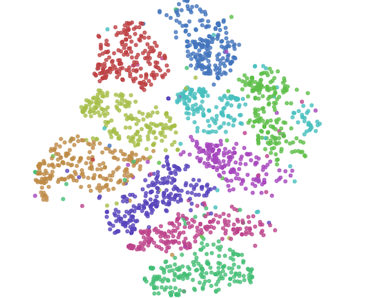
Intuitive在模型特征的选择时尤为重要,有效的数据可视化往往使得接下来的工作事半功倍。本文中的数据集只是简单的二维数据集,可视化自然不成问题,对于高纬数据,往往需要一个降维的过程,如基本的PCA,或者是hinton大神的t-SNE,其在Mnist高纬数据集的可视化效果非常赞:
 同时推荐一个非常不错的Machine Learning领域的数据可视化博客Colah's Blog。
。对该数据集我们可以画一个简单的二维数据分布图:
同时推荐一个非常不错的Machine Learning领域的数据可视化博客Colah's Blog。
。对该数据集我们可以画一个简单的二维数据分布图:
# STEP: 1: plot the data
X_axis, Y_axis = data.T[0], data.T[1]
plt.plot(X_axis, Y_axis, 'bo', label='Real data')
plt.ylim([0, 150])
plt.xlim([0, 45])
plt.legend()
plt.show()
分布如下所示:
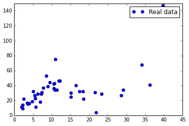
大致来看,数据集分布可以用一个简单的线性回归来适配,也可以整一个Quadratic函数来建模,当然此处为了演示线性回归,便先用线性回归来做。我们简单的选取模型为
Y = weight * X + bias
3.定义placeholder
既然模型确定了,我们便可以用TensorFlow的语言来定义模型图结构。placeholder是一种预先声明的function用来填充训练数据集的。对于线性回归而言,placeholder就是指X,Y,是来自测试数据集的,其不需要进行初始化,也不需要进行模型训练,只是在session run时feed真实的数据即可。
# STEP 2: create placeholder for input X(number of fire) and label Y(number of theft)
X = tf.placeholder(tf.float32, name="X")
Y = tf.placeholder(tf.float32, name="Y")
4. 定义Variable
相对于placeholder,Variable略为不同,前面一篇我们单独介绍过Variable的一些operation和属性。我们可以和placeholder来做个简单的对比,
| Name | placeholder | Variable |
|---|---|---|
| type | function | Class |
| 初始化 | NO | YES |
| 模型训练更新 | NO | YES |
| 存储 | 数据集群 | 参数服务器(PS) |
Stack Overflow上有个关于两者区别的讨论值得一看。
# STEP 3: create Variables(weight and bias here), initialize to 0.
w = tf.Variable(0.0, name="weight")
b = tf.Variable(0.0, name="bias")
5. 构建模型
这步很简单,依据第二部我们的模型选择,把其转换成Python表达,值得注意的是,由于是矩阵运算,如果X是高纬特征需要稍微考虑各个元素之间的位置。
# STEP 4: construct model to predict Y
Y_Predict = X * w + b
6. 定义损失函数
损失函数(loss function)的选择直接影响模型的训练复杂度和泛化效果。如针对linear regression最常见得损失函数式mean square error loss,即平方差损失。这种损失函数简单易用,但由于针对所有样本进行损失累计,一些outlier的点往往对整体模型有很大的影响,类似缺点的损失函数如absolute loss
The squared loss function results in an arithmetic mean-unbiased estimator, and the absolute-value loss function results in a median-unbiased estimator (in the one-dimensional case, and a geometric median-unbiased estimator for the multi-dimensional case). The squared loss has the disadvantage that it has the tendency to be dominated by outliers—when summing over a set of samples, the sample mean is influenced too much by a few particularly large a-values when the distribution is heavy tailed: in terms of estimation theory, the asymptotic relative efficiency of the mean is poor for heavy-tailed distributions. -wikipedia
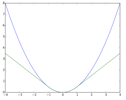
。还有一种叫做hubor loss的损失函数,相比于square error,其通过对偏离mean的点进行一定程度的loss惩罚(把损失近似成线性),使得
其对噪声样本(如离均值比较远的点)比较多的数据集有很好的效果。其和mean loss对比图一目了然:
# STEP 5: define loss function(use square error here)
# hubor_loss = tf.losses.huber_loss(Y, Y_Predict) for Hubor loss.
loss = tf.square(Y - Y_Predict, name="loss")
7. 定义Optimizer
一个算法模型最终能否转化成实际可用的industry工程实践,很大程度上区别于在现有computer power下的优化算法优劣。机器学习的很多模型都是non-determinate的算法,损失函数也可能是non-convex的,比如可能存在local optimization的问题,这时候优化方法便至关重要。TensorFlow提供了一大坨Optimizers,比如:
- tf.train.Optimizer
- tf.train.GradientDescentOptimizer
- tf.train.AdadeltaOptimizer
- tf.train.AdagradOptimizer
- tf.train.AdagradDAOptimizer
- tf.train.MomentumOptimizer
- tf.train.AdamOptimizer
- tf.train.FtrlOptimizer
- tf.train.ProximalGradientDescentOptimizer
- tf.train.ProximalAdagradOptimizer
- tf.train.RMSPropOptimizer
每一个算法都值得讲好几章有么有,以后有时间会一一研究下,有篇总结的帖子可以参考下。简而言之,梯度下降有两个问题,1)可能会陷入局部最优。2)依赖于learning rate的设置 而这两点在针对一些特定数据集(如stock market的稀疏数据)的条件下可能会导致模型找不到(或者在一定的epoch内)找不到最优解。这里对于简单的mean square loss,一般选择梯度下降就够了。
# STEP 6: define optimizer(here we use Gradient Descent with learning rate of 0.001)
optimizer = tf.train.GradientDescentOptimizer(learning_rate=0.001).minimize(loss)
8. 初始化与模型训练
到这里我们的基本模型定义已经完成,便需要设定一些基本的常量,或者对之前的Variable进行初始化。前一章节也大篇幅介绍了初始化的几种方法,再次不再赘述。初始化完毕便可以开始模型训练。模型定义完成后,模型的执行也基本是一行代码的事,唯一需要做的便是在Session里run时进行feed数据。
# define the epoch
epoch = 200
init = tf.initialize_all_variables()
# execute the model
with tf.Session() as sess:
    # STEP 7: initailize the necessary variable, in this case w and b.
    sess.run(init)

    # STEP 8: traning the model
    for i in range(epoch):
        for x, y in data:
            sess.run(optimizer, feed_dict={X: x, Y: y})

    # STEP 9: output the values of w and b.
    w_value, b_value = sess.run([w, b])
9. 效果评估与预测
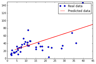
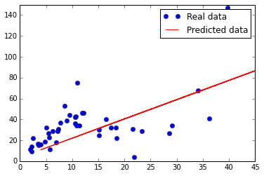
训练出来的模型适配原始的数据集如下所示,第一幅图是采用square error的线,第二幅是采用hubor loss的线,可以看出对于outlier点有了很好的规避。
# plot the predict line.
plt.plot(Y_axis, Y_axis * w_value + b_value, 'r', label='Predicted data')
plt.ylim([0, 150])
plt.xlim([0, 45])
plt.legend()
plt.show()