Linear Regression聊完了,自然就来到了Logistics Regression了。前者是预测一个连续的值,而后者是预测离散的值。前者的model是简单的线性特征组合,后者是在前者基础上加了一层sigmoid(通常二分类)或者softmax(多分类)的激活函数。因而对于模型loss的评估,连续值使用的如MSE(Mean Square Error),Huber;而后者则是离散的0-1之间的概率值,通常的损失函数为Cross Entropy和Hinge。因此Logistic Regression更general的来讲,其应该是Softmax Regression.
1.数据集获取与预处理
本文的测试数据是MNIST的手写数字字符,Tensorflow提供了直接的util类来下载数据集使用,但是天朝的网络通常是Request Timeout。所以这里直接通过翻墙或是啥的下载到工作目录最为省心。
# 数据集file主要有
weheng@34363bca98b0 ~/D/w/m/t/d/c/d/mnist> ls
t10k-images-idx3-ubyte.gz  t10k-labels-idx1-ubyte.gz  train-images-idx3-ubyte.gz train-labels-idx1-ubyte.gz
# 针对下面的数据直接使用wget获取即可
wget http://yann.lecun.com/exdb/mnist/{$file}
然后就开始数据读取,全局变量设置
import tensorflow as tf
from tensorflow.examples.tutorials.mnist import input_data

# reset everything to rerun in jupyter
tf.reset_default_graph()
tf.summary.FileWriterCache.clear()

# read data request timeout, could download to localhost first.
mnist = input_data.read_data_sets("data/mnist", one_hot=True)

learning_rate = 0.01
batch_size = 128
n_epoches = 25
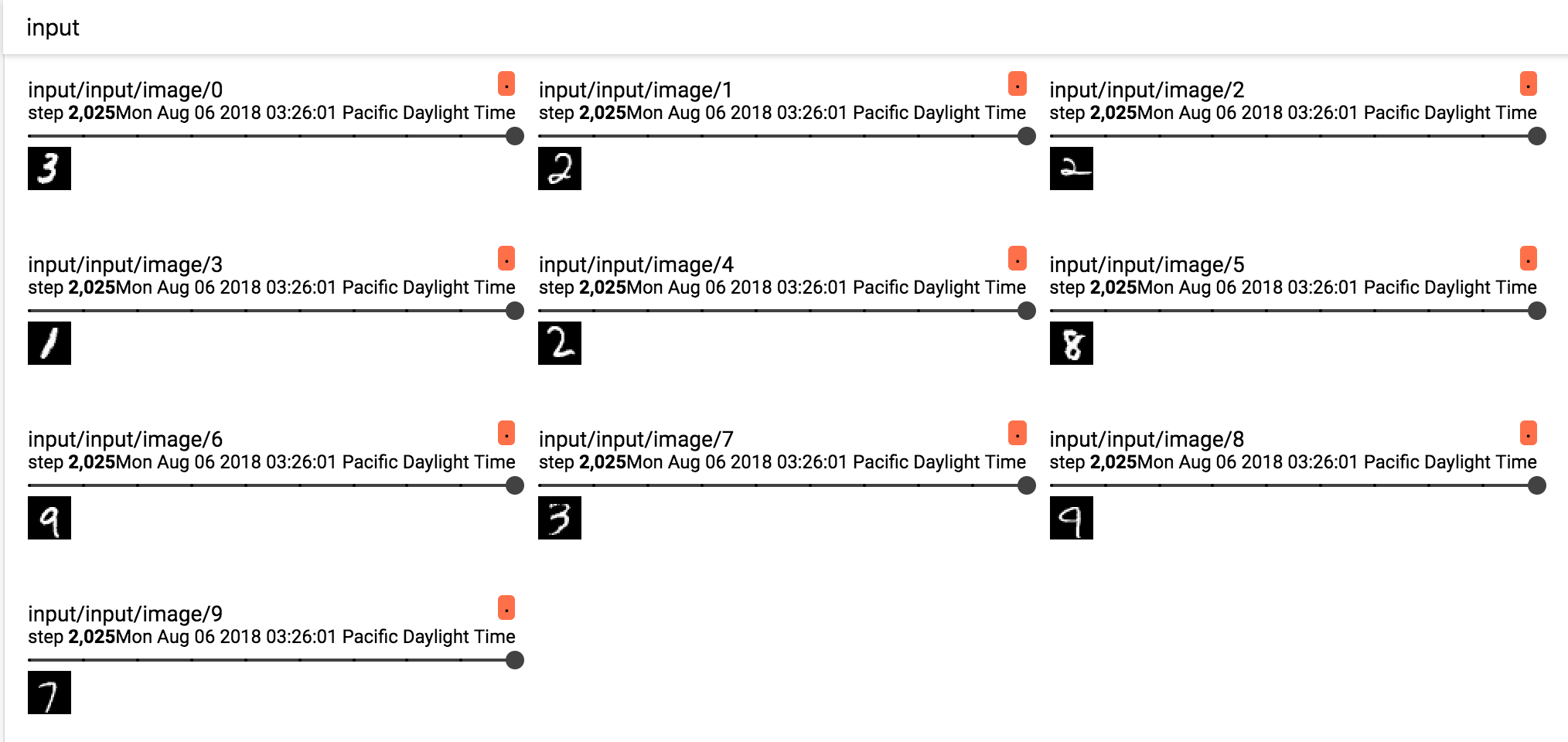
这里提到的是对于image数据,我们同样可以通过可视化工具来对其有个直观的印象。
2.输入数据可视化
我们可以通过可视化来简单直观的了解下MNIST数据集。记得我们之前介绍过Tensorboard,用其tf.summary.image的方法也可以进行数据可视化。
# input name space for tensorboard.
with tf.name_scope('input'):
    X = tf.placeholder(tf.float32, [batch_size, 784], name="image")
    Y = tf.placeholder(tf.float32, [batch_size, 10], name="label")
    image_shaped_input = tf.reshape(X, [-1, 28, 28, 1])
    tf.summary.image('input', image_shaped_input, 10)
如简单的数据可视化如下:
当然也可以直接在python里面,利用matplotlib来进行:
import tensorflow as tf
from tensorflow.examples.tutorials.mnist import input_data
import numpy as np
from matplotlib import pyplot as plt

# read data request timeout, could download to localhost first.
mnist = input_data.read_data_sets("data/mnist", one_hot=True)
first_image = mnist.test.images[0]
first_image = np.array(first_image, dtype='float')
pixels = first_image.reshape([28, 28])
plt.imshow(pixels, cmap=plt.get_cmap('gray_r'))
plt.show()
3.模型选择与变量定义
Softmax Regression(SR)本质是一种多分类的Logistic Regression(LR),不同点在于SR通常要求各个类别要求互斥(Mutually Exclusive)但不一定需要独立(Independent),而如果用LR来分类则要求独立,但不一定互斥。因此对于不同的分类任务,模型选择不同。这里的手写数字识别分类数据集中,一张图片通常只能有一个结果,损失函数便可以用softmax假设分类效果要好些,而如果数据集中出现了多章digtial数字,则可以考虑Logistic来做。听着有些晕,其实很直白的理解就是SR的函数表达更像是多个变量条件下的边际分布,而多分类情况下的LR,则是一种一对多的条件分布。
3.1 定义Weight和Bias
# train variables name space.
with tf.name_scope('weight'):
    w = tf.Variable(tf.random_normal(shape=[784, 10], stddev=0.01), name="weight")

with tf.name_scope('bias'):
    b = tf.Variable(tf.zeros([1, 10]), name="bias")
3.2 定义logit和loss函数
Wiki对logic的定义如下:
The logit of a number p between 0 and 1 is given by the formula:

在这里,这个number p很明显就是指linear regression里的这条直线wX + b。有了logit之后便可以针对softmax Regression使用cross entropy的损失函数。
with tf.name_scope('logits'):
    logits = tf.matmul(X, w) + b

# use softmax cross entropy with logits as the loss function
# compute the mean cross entropy, softmax is applied internally.
with tf.name_scope('entropy'):
    entropy = tf.nn.softmax_cross_entropy_with_logits(logits=logits, labels=Y)

# normalize step.
with tf.name_scope('loss'):
    loss = tf.reduce_mean(entropy)
定义预测metric和Optimizer
# can move accuracy into defintion, and put into optimizer in sess.run then.
with tf.name_scope('predict'):
    correct_preds = tf.equal(tf.argmax(logits, 1), tf.argmax(Y, 1))
    accuracy = tf.reduce_mean(tf.cast(correct_preds, tf.float32))

optimizer = tf.train.GradientDescentOptimizer(learning_rate=learning_rate).minimize(loss)
全局初始化与模型训练
# scalar for tensorboard.
tf.summary.scalar("cost", loss)
tf.summary.scalar('accuracy', accuracy)

summary_op = tf.summary.merge_all()

init = tf.global_variables_initializer()

with tf.Session() as sess:
    writer = tf.summary.FileWriter('./graphs', sess.graph)
    sess.run(init)
    # training the batch
    n_batches = int(mnist.train.num_examples/batch_size)
    for i in range(n_epoches):
        avg_cost = 0.
        for _ in range(n_batches):
            X_batch, Y_batch = mnist.train.next_batch(batch_size)
            _, l, summary = sess.run([optimizer, loss, summary_op], feed_dict={X: X_batch, Y:Y_batch})

            # Compute average loss
            avg_cost += l / n_batches

            # write log
            writer.add_summary(summary, n_epoches * n_batches + i)
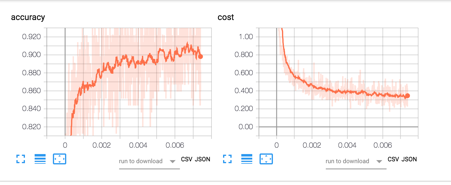
前面提到过,把一些变量进行一定规则的tf.name_scope命名以及tensorboard的使用,对于可视化训练过程和一些变量的变化趋势特别的有好处。例如上面我们把cost和accuracy加入可视化,便可以通过tensorboard来直观的看到训练过程中损失函数和精度随着训练样本数,次数的变化趋势,如下图所示:
效果评估与测试
根据tensorboard的预测效果进行参数(learning_rate, epoches,甚至是optimizer的有效调节),最后确定下比较满意的学习效果,然后便可以在测试集上进行测试。
# testing the model
    n_batches = int(mnist.test.num_examples/batch_size)
    for i in range(n_batches):
        X_batch, Y_batch = mnist.test.next_batch(batch_size)
        _, acc, summary = sess.run([optimizer, accuracy, summary_op], feed_dict={X: X_batch, Y: Y_batch})
        # write log
        writer.add_summary(summary, n_epoches * n_batches + i)
So long, and thanks for all the fish.
参考
[1] Tensorflow for Deep Learning Research.
[2] how-to-use-tensorboard.
[3] Softmax Regression.
[4] not-another-mnist-tutorial-with-tensorflow